Page 46 - ENGLISH_Housing
P. 46

Appendix III:


                                             Homeownership Rate


                                             and Housing Prices


                                                      As discussed in Chapter 8, there have been concerns that an in-
                                               crease in homeownership upon the privatisation of public housing under
                                               the proposed SHS might trigger undesirable fluctuations in the property
                                               market. This unease warrants further study.

                                               Methodology


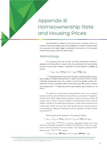
                                                      To investigate into this concern, we have conducted a panel re-
                                               gression with fixed effect to explore the nexus between homeownership
                                               rate and home prices variation.  Movement of home prices is modelled as
                                               follows:
                                                                                          •• ••••
                                                                       •• ••
                                                         •••••• •••• •••••••• •••••••••••••• •••••• •• •••• ••••
                                                                   ••
                                                                                                  ••••
                                                             ••••
                                                                                     ••••
                                                                                             ••
                                                                          ••••
                                                          ••••represents the home price indicator, measuring the percent-
                                                      ••••••
                                               age changes of residential properties in a given economy i  at time t, where
                                              t  denotes a particular year. X  is a vector of economy-specific control vari-
                                               ables that would conceivably affect home prices, e.g. GDP growth, inflation
                                               and interest rate ••••••   denotes the homeownership rate of economy i  at
                                                                  ••••
                                               time t..
                                                      To control for any omitted characteristics which are constant
                                               across economy yet are different across time, e.g. evolution of regulatory
                                               environment which might impact a group of nearby economy equally at
                                               a given year, a vector of binary variables Y representing different years is
                                               added. It equals 1 if the observation belongs to a given year, and is set to be
                                                         7
                                               0 otherwise . Finally, the error •• ••••••••  captures an economy-specific
                                                                                   ••••
                                                                                ••
                                                                           ••••
                                                                        ••
                                               time-invariant component •• and an economy-specific and time-variant
                                               component  ••   .
                                                           ••••
                                                      Rewriting the above equation in time period t-1 gives:
                                                                                            •• ••••
                                                                     •• ••
                                                    •••••• •••••••• •••• •••••• •••••••• •••••••• •••••••••••••• •••••••• •••••••••• •••••• ••••••••
                                                                                               ••••••
                                                            ••
                                                                            .
                                                                     ••
                                                      where  •••••••• •••••••• •••••••• . A panel regression model with fixed
                                               effect is numerically equivalent to taking a first difference of the two equa-
                                               tions, i.e. the two states of the economies in two adjacent periods of time.
                                                         •••••• ••••••••
                                               Differencing   ••••   ••••••••yields:
                                                                     •••••••••••• ••
                                                                                           •••••••••••• ••••
                                                     •••••••• •••••• •••••••••• •••••••••••••••• ••••••••••••••••••••
                                                                                                      ••••
                                                                                                ••••
                                                                 ••
                                                                                      ••••
                                                                          ••••
                                                          ••••
              7.  For example, if the observation is in the year 2004, then the variable representing the year 2004 will be set to 1, whereas
                 those representing the years 2005 to 2014 will be set to 0.
                                                                                                                  51
   41   42   43   44   45   46   47   48   49   50   51